 University of Padova
 University of Hawaii
 University of Lübeck
 arXiv Preprints
 ResearchGate
We briefly present graph wedgelets - a tool for data compression on graphs based on the representation of signals by piecewise constant functions on adaptively generated binary wedge partitionings of a graph. Graph wedgelets are discrete variants of continuous wedgelets and binary space partitionings known from image processing. We will see that wedgelet representations of graph signals can be encoded in a simple way and applied easily to the compression of graph signals and images.
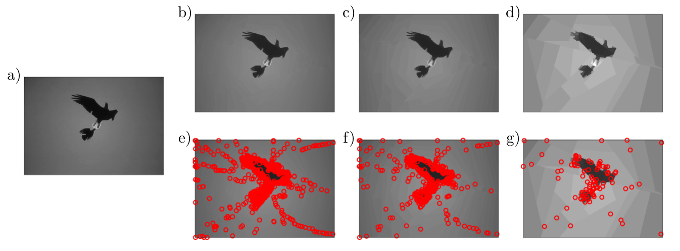
Fig. 1: Graph wedgelet compression of images. a) original image with $481 \times 321$ pixels; b)c)d) BWP compression with $1000$, $500$ and $100$ graph wedgelets; e)f)g) center nodes for BWP encoding in b)c)d). The PSNR values are b) 40.762 dB, c) 37.935 dB, and d) 31.827 dB.
1. Graphs and graph signals
We are interested in a sparse representation and compression of graph signals in terms of piecewise constant functions on adaptively generated graph partitionings. We will investigate signals on simple connected graphs $G=(V,E,\mathbf{A},\mathrm{d})$ with the following structural components:
- A set $V=\{\node{v}_1, \ldots, \node{v}_{n}\}$ consisting of $n$ graph vertices.
- A set $E \subseteq V \times V$ containing all edges $e_{i,i'} = (\node{v}_i, \node{v}_{i'})$, $i \neq i'$, of the graph $G$. We will assume that $G$ is undirected.
- A symmetric adjacency matrix $\Aa \in \Rr^{n \times n}$ with \begin{equation*} \displaystyle {\begin{array}{ll}\; \Aa_{i, i'}>0& \text{if $i \neq i'$ and $\node{v}_{i}, \node{v}_{i'}$ are connected by an edge,} \\ \; \Aa_{i, i'}=0 & \text{else.}\end{array}} \end{equation*} The positive non-diagonal elements $\Aa_{i, i'}$, $i \neq i'$, of the adjacency matrix $\Aa$ contain the connection weights of the edges $e_{i, i'} \in E$.
- The graph geodesic distance $\mathrm{d}$ on the vertices $V$, i.e., the length of the shortest path connecting two graph nodes. The distance $\mathrm{d}$ satisfies a triangle inequality and defines a metric on $V$.
Graph signals are functions $x: V \rightarrow \mathbb{R}$ on the vertex set $V$ of the graph $G$. As the vertices in $V$ are ordered, we can represent every signal $x$ also as a vector $x = (x(\node{v}_1), \ldots, x(\node{v}_n))^{\intercal}\in \mathbb{R}^n$. We can endow the space of all signals with the inner product \begin{equation*} y^\intercal x := \sum_{i=1}^n x(\node{v}_i) y(\node{v}_i). \end{equation*} In this way, we obtain a Hilbert space $\mathcal{L}^2(V)$ with the norm $\|x\|_{\mathcal{L}^2(V)}^2 = x^\intercal x$.
2. Binary wedge partitioning trees (BWP trees) on graphs
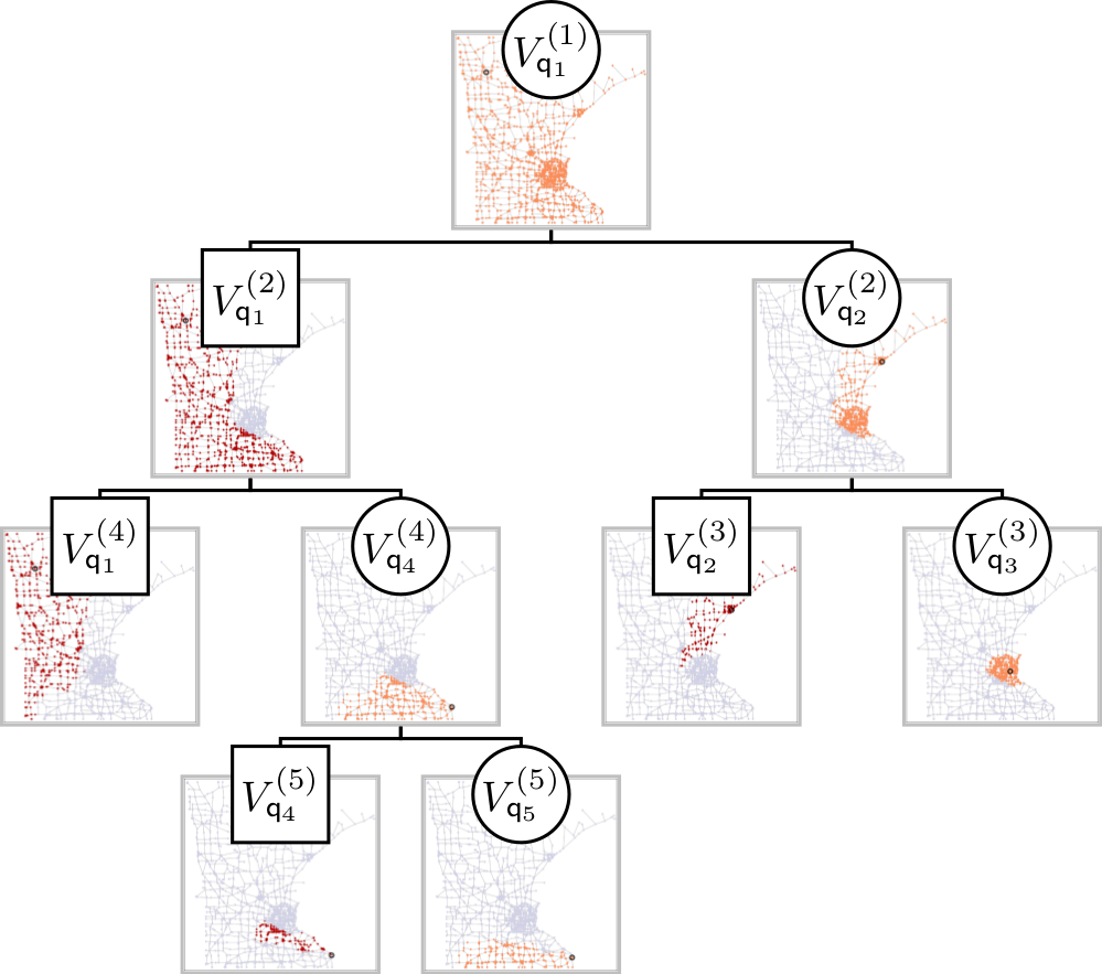
Fig. 2: A BWP tree for the adaptive approximation of a function on the Minnesota graph.
Wedgelet compression of graph signals relies on the adaptive recursive partitioning of the graph encoded in a tree structure. The binary partitioning trees for wedgelets are based on the following elementary wedge splits of vertex sets.
Definition 1. We call a dyadic partition $\{V', V''\}$ of the vertex set $V$ a wedge split of $V$ if there exist two distinct nodes $\node{v}'$ and $\node{v}''$ of $V$ such that $V'$ and $V''$ have the form \begin{align*} V' &= \{\node{v} \in V \ | \ \mathrm{d}(\node{v},\node{v}') \leq \mathrm{d}(\node{v},\node{v}'')\}, \quad \text{and} \\ V'' &= \{\node{v} \in V \ | \ \mathrm{d}(\node{v},\node{v}') > \mathrm{d}(\node{v},\node{v}'')\}. \end{align*}
A key advantage of the just defined elementary wedge splits is that they can be encoded very compactly by using only the two nodes $\node{v}' \in V'$ and $\node{v}'' \in V''$. Wedge splits have the following basic properties:
- $V'$ and $V''$ are uniquely determined by $\node{v}'$ and $\node{v}''$.
- $V' \cap V'' = \emptyset$ and $V' \cup V'' = V$.
- If the vertex set $V$ is connected, then also $V'$ and $V''$ are connected subsets of the graph $G$.
Using wedge splits, we can define elementary wedgelets as the functions \begin{align*} \omega_{(\node{v}',\node{v}'')}^{+} (\node{v}) &= \chi_{V'}(\node{v}) = \left\{\begin{array}{ll} 1, & \text{if $\mathrm{d}(\node{v},\node{v}') \leq \mathrm{d}(\node{v},\node{v}'')$}, \\ 0, & \text{otherwise}, \end{array} \right. \\ \omega_{(\node{v}',\node{v}'')}^{-} (\node{v}) &= \chi_{V''}(\node{v}) = \left\{\begin{array}{ll} 1, & \text{if $\mathrm{d}(\node{v},\node{v}') > \mathrm{d}(\node{v},\node{v}'')$}, \\ 0, & \text{otherwise}, \end{array} \right. \end{align*} where $\chi_{V'}$ and $\chi_{V''}$ denote the indicator functions of the sets $V'$ and $V''$, respectively. Wedge splits allow to generate the following binary partitioning trees for the graph $G$.
Definition 2. A binary wedge partitioning (BWP) tree $\mathcal{T}_Q$ of the graph $G$ with respect to the ordered set $Q = \{\node{q}_1, \ldots, \node{q}_M\} \subset V$ is a binary tree consisting of subsets of $V$ that can be ordered recursively in partitions $\mathcal{P}^{(m)}$, $m \in \mathbb{N}$, of $V$ by the following rules:
- The root of the tree $\mathcal{T}_Q$ is the entire set $V$ forming the trivial partition $\mathcal{P}^{(1)} = \{V_{\node{q}_1}^{(1)}\} = \{V\}$. The root is associated to the first node $\node{q}_1$ of $Q$.
- Let $\mathcal{P}^{(m)} = \{ V_{\node{q}_1}^{(m)}, \ldots, V_{\node{q}_m}^{(m)} \}$ be a partition of $V$ in the tree $\mathcal{T}_Q$ associated to the nodes $\node{q}_i \in V_{\node{q}_i}^{(m)}$, $i \in \{1, \ldots, m\}$, $m < M$. Consider now the point $\node{q}_{m+1} \in V_{\node{q}_j}^{(m)}$ for a $j \in \{1, \ldots, m\}$. We split the subset $V_{\node{q}_j}^{(m)}$ by a wedge split based on the nodes $\node{q}_{j}$ and $\node{q}_{m+1}$ into two disjoint sets $V_{(\node{q}_j,\node{q}_{m+1})}^{(m) \, +}$ (containing $\node{q}_j$) and $V_{(\node{q}_j,\node{q}_{m+1})}^{(m) \, -}$ (containing $\node{q}_{m+1}$) and obtain the new partition $$ \mathcal{P}^{(m+1)} = \{ V_{\node{q}_1}^{(m+1)}, \ldots, V_{\node{q}_{m+1}}^{(m+1)} \}$$ with $V_{\node{q}_i}^{(m+1)} = V_{\node{q}_i}^{(m)}$ if $i \neq \{j,m+1\}$, $V_{\node{q}_j}^{(m+1)} = V_{(\node{q}_j,\node{q}_{m+1})}^{(m) \, +}$ and $V_{\node{q}_{m+1}}^{(m+1)} =V_{(\node{q}_j,\node{q}_{m+1})}^{(m) \, -}$.
We call a BWP tree $\mathcal{T}_Q$ balanced if there exists $\frac12 \leq \rho < 1$ such that for every child $W'$ of an element $W \in \mathcal{T}_Q$ we have \[(1-\rho) |W| \leq |W'| \leq \rho |W|.\] We call a BWP tree $\mathcal{T}_Q$ complete if it has $n$ leaves, each containing a single vertex of the graph $G$.
A BWP tree $\mathcal{T}_Q$ is uniquely determined by the ordered set $Q$ of graph vertices. This allows to store the entire tree very compactly in terms of the $M$ elements of the set $Q$. In the next proposition, we sum up several basic properties of BWP trees. An example of a BWP tree of the Minnesota graph is given in Fig. 2.
Proposition 3. Let $\mathcal{T}_Q$ be a BWP tree determined by the ordered node set $Q = \{\node{q}_1, \ldots, \node{q}_M\}$.
- A BWP tree $\mathcal{T}_Q$ contains $2M -1$ elements: $1$ root and $2M - 2$ children.
- The $M$ leaves of the binary tree $\mathcal{T}_Q$ are given by the elements of the $M$-th. partition $\mathcal{P}^{(M)} = \{ V_{\node{q}_1}^{(M)}, \ldots, V_{\node{q}_{M}}^{(M)}\}$.
- A BWP tree $\mathcal{T}_Q$ is complete if and only if $|Q| = |V|$.
- A BWP tree $\mathcal{T}_Q$ is balanced with \[ \frac12 \leq \rho \leq \frac{n-1}{n}.\]
- The characteristic function of the subset $V_{\node{q}_i}^{(m)}$ can be written as a product of $m$ elementary wedgelets $\omega_{(\node{q}_i,\node{q}_j)}^{\pm}$, with $\node{q}_i, \node{q}_j \in \{\node{q}_1, \ldots, \node{q}_m\}$, $i < j$.
Definition 4. The indicator functions \[\omega_{\node{q}_i}^{(m)}(\node{v}) = \chi_{V_{\node{q}_i}^{(m)}}(\node{v}), \quad 1 \leq i \leq m, \; 1 \leq m \leq M,\] of the sets $V_{\node{q}_i}^{(m)}$ will be referred to as wedgelets with respect to the BWP tree $\mathcal{T}_Q$. The wedgelets $\{\omega_{\node{q}_i}^{(m)}\,:\,1 \leq i \leq m\}$ form an orthogonal basis for the piecewise constant functions on the partition $\mathcal{P}^{(m)}$, using the standard inner product in the space $\mathcal{L}^2(V)$.
3. Greedy generation of BWP trees
To generate a BWP tree $\mathcal{T}_Q$, at each partition stage $m$ one of the subdomains $V_{\node{q}_j}^{(m)}$, $j \in \{1, \ldots, m\}$, has to be chosen. Moreover, a new node $\node{q}_{m+1} \in V_{\node{q}_j}^{(m)}$ is required to perform the consequent elementary wedge split of the set $V_{\node{q}_j}^{(m)}$. For a graph signal $f$ to be approximated, both choices can be made in an $f$-adapted way or in a non-adaptive way. We will consider the following three greedy methods for this procedure:
Max-distance (MD) greedy wedge splitting. At stage $m$, the domain $V_{\node{q}_j}^{(m)}$ is chosen to be the one for which the $\mathcal{L}^2$-error is maximal, i.e., the index $j$ is determined as \begin{equation} \tag{1} j = \underset{i \in \{1, \ldots, m\}}{\mathrm{argmax}} \|f - \bar{f}_{V_{\node{q}_i}^{(m)}}\|_{\mathcal{L}^2(V_{\node{q}_i}^{(m)})},\end{equation} where \[\bar{f}_{V_{\node{q}_i}^{(m)}} = \frac{\langle f, \omega_{\node{q}_i}^{(m)} \rangle}{|V_{\node{q}_i}^{(m)}|} = \frac{1}{|V_{\node{q}_i}^{(m)}|} \sum_{\node{v} \in V_{\node{q}_i}^{(m)}} f(\node{v})\] denotes the mean value of $f$ over the set $V_{\node{q}_i}^{(m)}$. As soon as $j$, or equivalently, $\node{q}_j$ are determined, a non-adaptive way to choose the subsequent node set $\node{q}_{m+1}$ is by the selection rule \[ \node{q}_{m+1} = \underset{\node{v} \in \in V_{\node{q}_j}^{(m)}}{\mathrm{argmax}} \, \mathrm{d}(\node{q}_j,\node{v}), \] i.e., $\node{q}_{m+1}$ is chosen to be the vertex furthest away from $\node{q}_j$ in $V_{\node{q}_j}^{(m)}$. This choice and the corresponding split can be interpreted as a two center clustering of $V_{\node{q}_j}^{(m)}$ in which the first node $\node{q}_j$ is fixed. One heuristic reason for this selection is that the resulting binary partitions in the BWP tree might be more balanced with a smaller constant $\rho$ compared to the theoretical upper bound $1 - 1/n$ in Proposition 3.
Fully adaptive (FA) greedy wedge splitting. In the FA-greedy procedure the subset $V_{\node{q}_j}^{(m)}$ to be split is selected as in (1), but also the node $\node{q}_{m+1}$ determining the wedge split is chosen according to an adaptive rule. If $\{ V_{(\node{q}_j,\node{q})}^{(m) \, +}, V_{(\node{q}_j,\node{q})}^{(m) \, -}\}$ denotes the partition of $V_{\node{q}_j}^{(m)}$ according to the wedge split given by the node $\node{q}_j$ and a second node $\node{q}$, we determine $\node{q}_{m+1}$ such that the $\mathcal{L}^2$-error \begin{equation} \tag{2} \left( \|f - \bar{f}_{V_{(\node{q}_j,\node{q})}^{(m) \, +}}\|_{\mathcal{L}^2(V_{(\node{q}_j,\node{q})}^{(m) \, +})}^2 + \|f - \bar{f}_{V_{(\node{q}_j,\node{q})}^{(m) \, -}}\|_{\mathcal{L}^2(V_{(\node{q}_j,\node{q})}^{(m) \, -})}^2 \right) \end{equation} is minimized over all $\node{q} \in V_{\node{q}_j}^{(m)}$. Compared to the semi-adaptive MD-greedy procedure, the FA-greedy method is computationally more expensive. On the other hand, as the wedge splits are more adapted to the particular form of the underlying function $f$, we expect a better approximation behavior for the FA-greedy scheme.
Randomized (R) greedy wedge splitting. If the size of the subsets $V_{\node{q}_j}^{(m)}$ is large it might be too time-consuming to find the global minimum of the $\mathcal{L}^2$-error (2) in the FA-greedy scheme. A quasi-optimal alternative to the fully-adaptive procedure is a randomized splitting strategy, in which the minimization of the $\mathcal{L}^2$-error (2) is performed on a subset of $1 \leq R \leq |V_{\node{q}_j}^{(m)}|$ randomly picked nodes of $V_{\node{q}_j}^{(m)}$. In this strategy, the parameter $R$ acts as a control parameter giving a result close or identical to FA-greedy if $R$ is chosen large enough.
We summarize the wedgelet encoding and decoding of a graph signal using a greedy-based binary wedge partitioning of the graph in Algorithm 1 and Algorithm 2.
Input: graph signal $f$, starting node $\node{q}_1 \in V$, starting partition $\mathcal{P}^{(1)} = \{V\} = \{V_{\node{q}_1}^{(1)}\}$, and final partition size $M \geq 1$.
For $m = 2$ to $M$ do
- Greedy selection of subset: calculate $j$ according to the rule (1) given as \[ j = \underset{i \in \{1, \ldots, m-1\}}{\mathrm{arg \, max}} \left\|f - \bar{f}_{V_{\node{q}_i}^{(m-1)}} \right\|_{\mathcal{L}^2(V_{\node{q}_i}^{(m-1)})};\]
- Conduct one of the following alternatives:
Max-distance (MD) greedy procedure: select new node $\node{q}_m = \underset{\node{v} \in V_{\node{q}_j}^{(m)}}{\mathrm{arg \, max}} \; \mathrm{d}(\node{q}_j,\node{w})$ farthest away from $\node{q}_j$ and add it to the node set $Q$;
Fully-adaptive (FA) greedy procedure: determine new node $\node{q}_m$ such that the squared $\mathcal{L}^2$-error term (2) is minimized and add it to the node set $Q$;
Randomized (R) greedy procedure: determine $\node{q}_m$ such that (2) is minimized over a subset of $R$ randomly chosen points and add it to $Q$;
- Generate the new partition $\mathcal{P}^{(m)}$ from the partition $\mathcal{P}^{(m-1)}$ by a wedge split of the subset $V_{\node{q}_j}^{(m-1)}$ into the children sets $V_{(\node{q}_j,\node{q}_{m})}^{(m-1) \, +}$ and $V_{(\node{q}_j,\node{q}_m)}^{(m-1) \, -}$;
- Compute mean values $\bar{f}_{V_{\node{q}_i}^{(m)}}$, $i \in \{1, \ldots, m\}$, for the new partition $\mathcal{P}^{(m)}$ by an update from $\mathcal{P}^{(m-1)}$.
Output: node set $Q = \{\node{q}_1, \ldots, \node{q}_{M}\}$ and mean values $\left\{\bar{f}_{V_{\node{q}_1}^{(M)}}, \ldots, \bar{f}_{V_{\node{q}_M}^{(M)}}\right\}$.
Input: node set $Q = \{\node{q}_1, \ldots, \node{q}_{M}\}$, and mean function values $\left\{\bar{f}_{V_{\node{q}_1}^{(M)}}, \ldots, \bar{f}_{V_{\node{q}_M}^{(M)}}\right\}$.
Calculate the partition $\mathcal{P}^{(M)} = \{V_{\node{q}_1}^{(M)}, \ldots, V_{\node{q}_M}^{(M)}\}$ of $V$ by elementary wedge splits along the BWP tree $\mathcal{T}_Q$ according to the recursive procedure in Definition 2.
Output: The wedgelet approximation \[\mathcal{W}_M f(\node{v}) = \sum_{i = 1}^M \bar{f}_{V_{\node{q}_i}^{(M)}} \, \omega_{\node{q}_i}^{(M)} (\node{v})\] of the graph signal $f$. For $M = n$, the original function $\mathcal{W}_n f = f$ is reconstructed.
4. Examples
As a first example graph, we consider the Minnesota graph, a road network of the state of Minnesota. This dataset consists of $n=2642$ vertices and $3304$ edges. As a test signal, we consider the binary function \[f(\node{v})) = 2 \chi_{W}(\node{v}) -1\] based on the characteristic function of the node sets \begin{align*} W &= \{\node{v} \in V \ | \ x_\node{v} <-94\}. \end{align*} Starting from a randomly chosen initial node $\node{q}_1$ we apply Algorithm 1 and Algorithm 2 to generate the BWP tree and a piecewise constant approximation of the function $f$. In Fig. 3, different approximations $\mathcal{W}_m f$ of the function $f$ are illustrated for different partitioning stages $m$ (we used FA-greedy to generate the BWP tree).
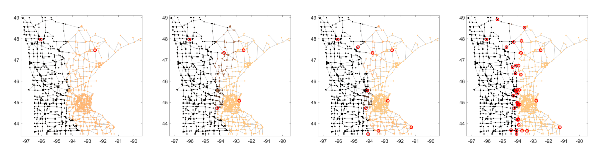
Fig. 3: Approximation of the binary signal $f$ on the Minnesota graph with $2,5,10$ and $40$ wedgelets (from left to right). The red rings indicate the center nodes $Q$. The number of wrongly classified nodes equals $356$, $286$, $110$, and $12$, respectively.
As adaptive partitioning tools for discrete domains, BWPs can also be used for the piecewise approximation and compression of images. An image can be naturally thought of as a finite rectangular grid of pixels and interpreted as a graph. Pixels close to each other are therein linked by a weighted edge. The structure and the weights of the single edges determine the local dependencies in the image and have therefore a strong influence on the outcome of the greedy algorithms. A simple qualitative comparison of the role of the metric $\mathrm{d}$ is given in Fig. 4. The $1$-norm and the infimum norm for the distance of the pixels lead to partitions with a rather rectangular or rhomboid wedge structure. On the other hand, wedges generated by the $2$-norm seem to be more anisotropic and slightly better adapted to the edges of the image.
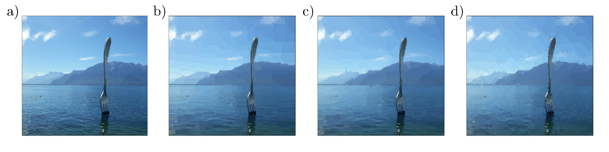
Fig. 4: Role of the metric in BWP compression a) original image with $500 \times 451$ pixels; b)c)d) R-greedy BWP compression using $M = 1000$ nodes, $R = 500$ as well as b) the $1$-norm, c) the $2$-norm and d) the infimum norm for the pixel distance.
We finally compare the performance of the FA-greedy and the MD-greedy method for the compression of images. In the example given in Fig. 5, we see that, as expected, the FA-greedy performs considerably better. In particular, the wavelet details in the FA-greedy scheme are smaller and more distinguished than for MD-greedy when using the same number of wedge splits. Regarding the distribution of the center nodes $Q$, we see further in Fig. 1 above that the adaptive BWP scheme (in this case a R-greedy scheme) selects the new nodes increasingly closer to the edges of the image such that most refinements of the partitions are performed in those regions where the gradients are large.
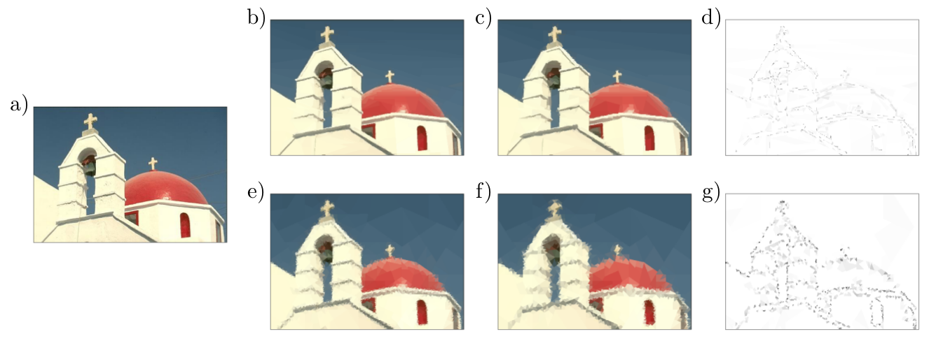
Fig. 5: BWP compression of images. a) original image with $481 \times 321$ pixels; b)c) FA-greedy BWP compression with $2000$ and $1000$ nodes; d) wavelet details between b) and c); e)f) MD-greedy BWP compression with $2000$ and $1000$ nodes; g) wavelet details between e) and f).
Main publications
- [1] Erb, W. Graph Wedgelets: Adaptive Data Compression on Graphs based on Binary Wedge Partitioning Trees and Geometric Wavelets. arXiv:2110.08843 (2021) (Preprint)
Software
- GraphWedgelets: A software package for the illustration of graph wedgelets in image compression.