Wolfgang Erb | Rhodonea curves

Fig. 1: Table of rhodonea curves for different frequencies $m_1$ (columns), $m_2$ (rows), and rotation angles $\alpha$.
(Applet adapted from: D. Shiffman, http://codingtra.in, coding challenge #116: Lissajous Curve Table)

Rhodonea curves are classical planar curves in the disk with the characteristic shape of a petalled rose. For this, they are also sometimes called rose curves or roses of Grandi, in honour of the monk and mathematician Guido Grandi who studied them intensively in the 18th century.

More concretely, for a frequency vector $\boldsymbol{m} = (m_1, m_2) \in{\mathbb N}^{2}$ and a rotation parameter $\alpha \in {\mathbb R}$, a rhodonea curve is given as \[\label{201509161237} \boldsymbol{\varrho}^{(\boldsymbol{m})}_{\alpha}(t) = \Big( \cos(m_2 t) \cos (m_1 t - \alpha \pi), \ \cos(m_2 t) \sin (m_1 t - \textstyle\alpha \pi) \Big), \quad t \in \mathbb{R}.\] In Fig. 1 and Fig. 2, some typical examples of such a curve are illustrated.

Fig. 2: The rhodonea curves $\boldsymbol{\varrho}^{(\boldsymbol{m})}_{\alpha}$ for different parameters $\boldsymbol{m} = (m_1, m_2)$ and $\alpha$.

In the following, we give a brief overview about rhodonea curves and, more generally, about rhodonea varieties, i.e., ensembles of rhodonea curves. The mathematical proofs of the statements can be found in [1]. We are particularly interested in the intersection points and boundary points of rhodonea curves, as these are interesting nodes for interpolation schemes on the disk.

1. General properties of rhodonea curves

As a first observation from Fig. 2, we see that the curve $\boldsymbol{\varrho}^{(\boldsymbol{m})}_{\alpha}$ is contained in the unit disk $\mathbb{D}= \{\boldsymbol{x} \in {\mathbb R}^2 \ : \ |\boldsymbol{x}| \leq 1\}$ and that the parameter $\alpha$ describes in fact a rotation of the curve in clockwise orientation. The frequency parameters $m_1$ and $m_2$ in the rhodonea curve $\boldsymbol{\varrho}^{(\boldsymbol{m})}_{\alpha}$ determine a superposition of a radial and an angular harmonic motion. For this reason, rose curves can also be regarded as polar variants of bivariate Lissajous curves. The time period to traverse the entire curve $\boldsymbol{\varrho}^{(\boldsymbol{m})}_{\alpha}(t)$ exactly one time depends on the parameters $m_1$ and $m_2$. If the frequencies $m_1$ and $m_2$ are relatively prime, then the period $P$ is given by $P=2\pi$ if $m_1+m_2$ is odd, and $P = \pi$ if $m_1+m_2$ is even. Depending on whether $m_1+m_2$ is even or odd, the behavior of $\boldsymbol{\varrho}^{(\boldsymbol{m})}_{\alpha}$ will vary slightly also with respect to other properties.

For a general parameter $\boldsymbol{m} \in {\mathbb N}^2$ and the greatest common divisor of $m_1$ and $m_2$ denoted with $g = \mathrm{gcd}(\boldsymbol{m}) \geq 1$, we can write $\boldsymbol{\varrho}^{(\boldsymbol{m})}_{\alpha}(t) = \boldsymbol{\varrho}^{(\boldsymbol{m}/g)}_{\alpha}( g t)$. In this case, the period of $\boldsymbol{\varrho}^{(\boldsymbol{m})}_{\alpha}$ is given by $P/g$. In particular, all properties of a rose $\boldsymbol{\varrho}^{(\boldsymbol{m})}_{\alpha}$ with general $\boldsymbol{m} \in {\mathbb N}^2$ can be obtained from the curve $\boldsymbol{\varrho}^{(\boldsymbol{m}/g)}_{\alpha}$ with the relatively prime parameter $\boldsymbol{m}/g$. When analyzing the properties of a single rose curve it is therefore enough to restrict the considerations to relatively prime frequency numbers $m_1$ and $m_2$. However, if more than one rhodonea curve is used to generate the interpolation nodes, also the general case plays an important role.

2. The self-intersection and boundary points of the rhodonea curves

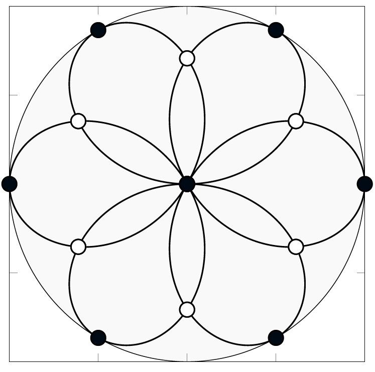
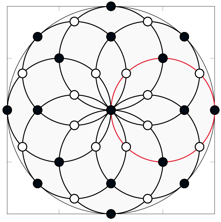
Fig. 3: Two rhodonea varieties with its intersection and boundary points. Left: The single rhodonea curve $\boldsymbol{\varrho}^{(2,3)}_{0}$ determines the rhodonea variety. Right: The rhodonea variety $\mathcal{R}^{(4,4)}$ consists of the eight rotated circles $\boldsymbol{\varrho}^{(4,4)}_{0}, \boldsymbol{\varrho}^{(4,4)}_{\pi/4 }, \boldsymbol{\varrho}^{(4,4)}_{2 \pi/4 }, \ldots, \boldsymbol{\varrho}^{(4,4)}_{7\pi/4}$.

For a first characterization of all self-intersection points of the curve $\boldsymbol{\varrho}^{(\boldsymbol{m})}_{\alpha}$, we consider for $t \in [0,2\pi)$ the sets $\mathcal{S}^{(\boldsymbol{m})}(t) = \{ s \in [0,2\pi): \ \boldsymbol{\varrho}^{(\boldsymbol{m})}_{\alpha}(s) = \boldsymbol{\varrho}^{(\boldsymbol{m})}_{\alpha}(t) \}$ and the sampling points \[\begin{aligned} t^{(\boldsymbol{m})}_{l} &= \frac{l \pi}{2 m_1 m_2}, \quad l \in \{0,1, \ldots, 4m_1m_2-1\}. \label{eq-samples1}\end{aligned}\]

Proposition 1 Let $m_1$ and $m_2$ be relatively prime numbers.
If $m_1+m_2$ is odd, the minimal time period of $\boldsymbol{\varrho}^{(\boldsymbol{m})}_{\alpha}$ is $P = 2 \pi$ and \[\begin{array}{lll} (i) & \# \mathcal{S}^{(\boldsymbol{m})}(t) = 2 m_2 & \text{if}\quad t \in \{\,t^{(\boldsymbol{m})}_{l}\,| \ l\in \{0,\ldots,4m_1m_2-1\}, \ l \equiv m_1 \mod 2 m_1 \},\\ (ii) & \# \mathcal{S}^{(\boldsymbol{m})}(t) = 2 & \text{if}\quad t \in \{\,t^{(\boldsymbol{m})}_{l}\,| \ l\in \{0,\ldots,4m_1m_2-1\}, \ l \not\equiv 0 \mod m_1 \}, \\ (iii) & \# \mathcal{S}^{(\boldsymbol{m})}(t) = 1 & \text{for all other $t \in [0,2\pi)$.} \end{array}\] If $m_1+m_2$ is even, then the minimal time period of $\boldsymbol{\varrho}^{(\boldsymbol{m})}_{\alpha}$ is $P = \pi$ and \[\begin{array}{lll} (i)' & \# \mathcal{S}^{(\boldsymbol{m})}(t) = 2 m_2 & \text{if}\quad t \in \{\,t^{(\boldsymbol{m})}_{l}\,| \ l\in \{0,\ldots,4m_1m_2-1\}, \ l \equiv m_1 \mod 2 m_1 \}, \\ (ii)' & \# \mathcal{S}^{(\boldsymbol{m})}(t) = 4 & \text{if}\quad t \in \{\,t^{(\boldsymbol{m})}_{2l}\,| \ l\in \{0,\ldots,2m_1m_2-1\}, \ l \not\equiv 0 \mod m_1 \}, \\ (iii)' & \# \mathcal{S}^{(\boldsymbol{m})}(t) = 2 & \text{for all other $t \in [0,2\pi)$.} \end{array}\]

We can extract a series of properties from this result. The nodes $\boldsymbol{\varrho}^{(\boldsymbol{m})}_{\alpha}(t)$ in $(i)$ and $(i)'$ with $\# \mathcal{S}^{(\boldsymbol{m})}(t) = 2 m_2$ correspond to the center $(0,0)$ of the unit disk $\mathbb{D}$. As $t$ varies from $0$ to $P$, the center is traversed $2m_2$ times in the case that $m_1+m_2$ is odd and $m_2$ times if $m_1+m_2$ is even. All the points $\boldsymbol{\varrho}^{(\boldsymbol{m})}_{\alpha}(t)$ in $(ii)$ and $(ii)'$ are doubly traversed in one period $P$. Therefore, if $m_1+m_2$ is odd, Proposition 1 ensures that the set \[\label{1709171731} \boldsymbol{\mathrm{RD}}^{(\boldsymbol{m})}_{\alpha} = \left\{\,\boldsymbol{\varrho}^{(\boldsymbol{m})}_{\alpha}(t^{(\boldsymbol{m})}_{l})\,|\, l\in \{0,\ldots,4m_1m_2-1\} \,\right\}\] contains all self-intersection points of the curve $\boldsymbol{\varrho}^{(\boldsymbol{m})}_{\alpha}$. The additional nodes $\boldsymbol{\varrho}^{(\boldsymbol{m})}_{\alpha}(t^{(\boldsymbol{m})}_{l})$ with $l \equiv 0 \mod 2 m_1$ describe precisely the set of all points at which the curve $\boldsymbol{\varrho}^{(\boldsymbol{m})}_{\alpha}$ touches the boundary of the unit disk $\mathbb{D}$ (i.e. the unit circle). If $m_1+m_2$ is even, the set $\boldsymbol{\mathrm{RD}}^{(\boldsymbol{m})}_{\alpha}$ is larger than the union of self-intersection and boundary points of $\boldsymbol{\varrho}^{(\boldsymbol{m})}_{\alpha}$. Nevertheless, also in this case the set $\boldsymbol{\mathrm{RD}}^{(\boldsymbol{m})}_{\alpha}$ will play an important role in our considerations. We summarize all important properties of the rhodonea curves in the following Corollary 2 and in Table 1 below.

Corollary 2 Let $m_1$ and $m_2$ be relatively prime natural numbers.

If $m_1 + m_2$ is odd, then $\boldsymbol{\mathrm{RD}}^{(\boldsymbol{m})}_\alpha$ is the union of all self-intersection and all boundary points of the closed curve $\boldsymbol{\varrho}^{(\boldsymbol{m})}_{\alpha}$. $\boldsymbol{\mathrm{RD}}^{(\boldsymbol{m})}_\alpha$ contains $2 m_1 m_2 + 1$ points in $\mathbb{D}$. It includes the center $(0,0)$ that is traversed $2 m_2$ times in one period $P = 2\pi$, $2 (m_1-1) m_2$ ordinary double points distinct from $(0,0)$ and $2m_2$ points on the boundary of $\mathbb{D}$.
If $m_1 + m_2$ is even, the curve $\boldsymbol{\varrho}^{(\boldsymbol{m})}_{\alpha}$ contains $\frac12(m_1-1) m_2$ ordinary double points distinct from $(0,0)$ and $m_2$ points on the boundary of $\mathbb{D}$. The center $(0,0)$ is traversed $m_2$ times in one period $P = \pi$.

Curve $\boldsymbol{\varrho}^{(\boldsymbol{m})}_{\alpha}$	Intersection points	Type of intersection points	Boundary points
$m_1 + m_2$ odd	$2(m_1-1) m_2 + 1$	$\begin{array}{l} \text{Center, traversed $2 m_2$ times in one period,} \\ \text{$2(m_1-1) m_2$ noncentric double points} \end{array}$	$2 m_2$
$m_1 + m_2$ even	$\frac12(m_1-1) m_2 + 1 $ if $ m_2 \neq 1 $ $\frac12(m_1-1) m_2 \phantom{+ 1 }\;\, $ if $ m_2 = 1 $	$\begin{array}{l} \text{Center, traversed $m_2$ times in one period,} \\ \text{$\frac12(m_1-1) m_2$ noncentric double points} \end{array}$	$m_2$

Table 1: Number of intersection and boundary points for the curve $\boldsymbol{\varrho}^{(\boldsymbol{m})}_{\alpha}$ if $m_1$, $m_2$ are relatively prime. For general $\boldsymbol{m}$, the corresponding numbers are obtained by considering the curve $\boldsymbol{\varrho}^{(\boldsymbol{m}/g)}_{\alpha}$ instead ($g = \mathrm{gcd}(\boldsymbol{m})$).

3. The rhodonea nodes as interlacing polar grids

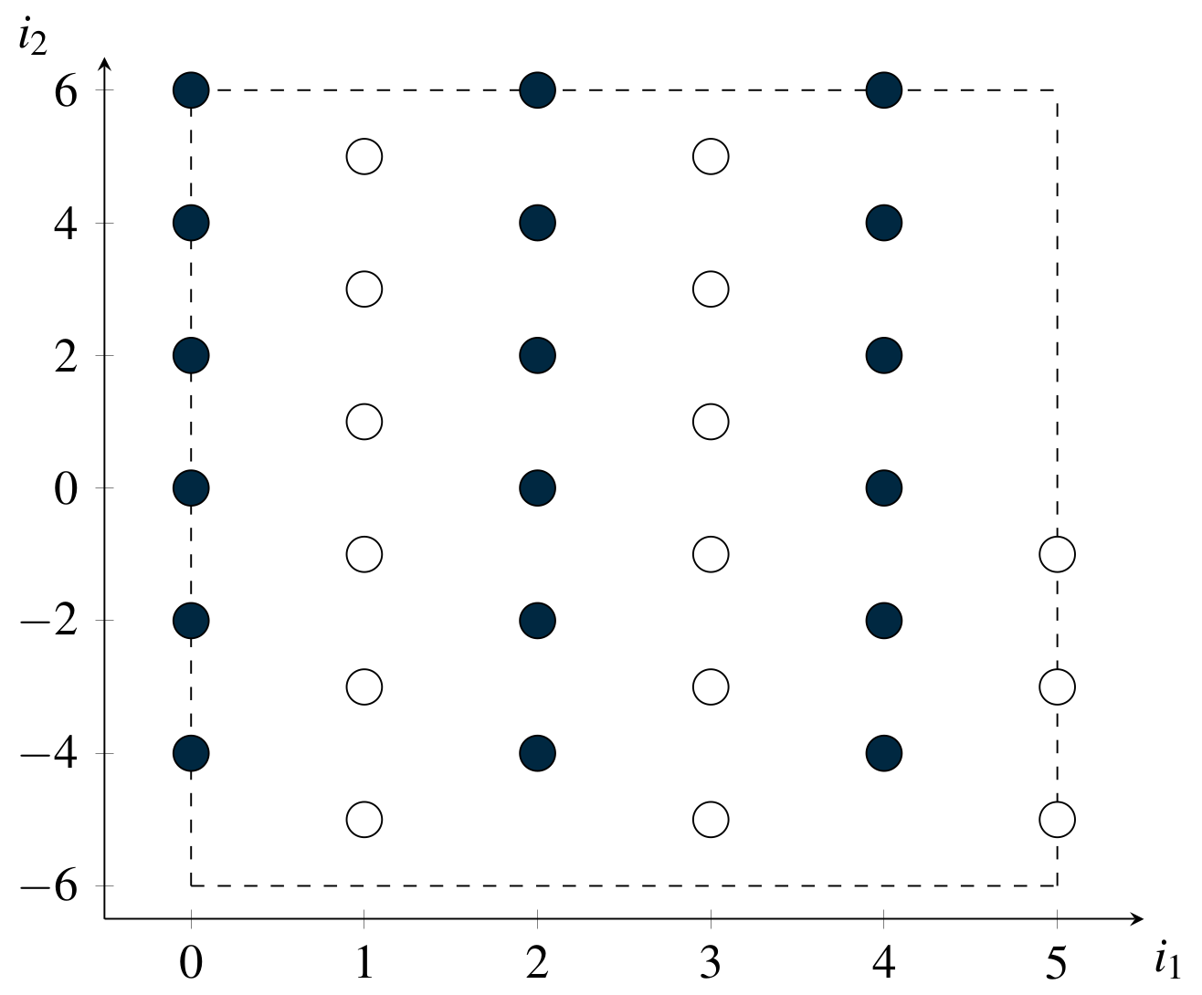
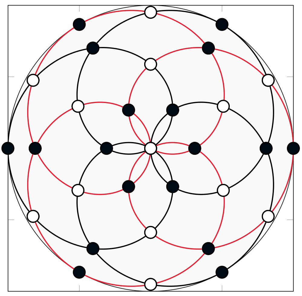
Fig. 4: Rhodonea nodes as disjoint union of polar grids. Left: the nodal index set for the rhodonea nodes. The indices on the left boundary are mapped onto the boundary of the disk, the indices on the right to the center. Right: the rhodonea nodes corresponding to the indices on the left together with the two generating rhodonea curves.

The nodes $\boldsymbol{\mathrm{RD}}^{(\boldsymbol{m})}_\alpha$ of the rhodonea curve $\boldsymbol{\varrho}^{(\boldsymbol{m})}_{\alpha}$ in the first part of Corollary 2 form a union of two interlacing rectangular grids in polar coordinates. This second description of the node points can be formulated for general frequencies $\boldsymbol{m} = (m_1, m_2) \in\mathbb{N}^{2}$.

To obtain this more general characterization, we introduce the nodal index set \[\label{eq:0911} \boldsymbol{\mathrm{I}}^{(\boldsymbol{m})}= \left\{ \,(i_1, i_2) \in {\mathbb Z}^{2}\ \left|\begin {array}{ll} & 0\leq i_{1}\leq m_{1}, \; -2 m_2 < i_2 \leq 2 m_2, \\ & \text{$i_2 \leq 0$ if $i_{1} = m_1$}, \\ & \text{$i_{1} + i_{2}$ is even} \end{array}\right. \, \right\}.\] The set $\boldsymbol{\mathrm{I}}^{(\boldsymbol{m})}$ can be decomposed into the two disjoint finite grids $\boldsymbol{\mathrm{I}}^{(\boldsymbol{m})}_0$ and $\boldsymbol{\mathrm{I}}^{(\boldsymbol{m})}_1$ given by \[\label{eq:0901} \boldsymbol{\mathrm{I}}^{(\boldsymbol{m})}_0 = \{(i_1, i_2) \in \boldsymbol{\mathrm{I}}^{(\boldsymbol{m})}\ | \ \text{$i_1$, $i_2$ are even} \, \}, \quad \boldsymbol{\mathrm{I}}^{(\boldsymbol{m})}_1 = \{(i_1, i_2) \in \boldsymbol{\mathrm{I}}^{(\boldsymbol{m})}\ | \ \text{$i_1$, $i_2$ are odd} \, \}.\] A tuple $\boldsymbol{i} = (i_1, i_2)$ in $\boldsymbol{\mathrm{I}}^{(\boldsymbol{m})}$ has a one to one relation to a point in polar coordinates by introducing a radial and an angular component \[r^{(m_1)}_{i_1} = \cos \left( \frac{i_1}{2 m_1} \pi \right) \in [0,1], \qquad \theta^{(m_2)}_{i_2} = \frac{i_2}{2 m_2} \pi \in (-\pi,\pi].\] The general rhodonea nodes on the unit disk are then defined as the point set \[\label{eq:09172} \boldsymbol{\mathrm{RD}}^{(\boldsymbol{m})}=\left\{\, \boldsymbol{x}^{(\boldsymbol{m})}_{\boldsymbol{i}}\,\left|\,\boldsymbol{i}\in \boldsymbol{\mathrm{I}}^{(\boldsymbol{m})}\right.\right\},\]

with the nodes $\boldsymbol{x}^{(\boldsymbol{m})}_{\boldsymbol{i}} \in \mathbb{D}$ given in polar coordinates $(r^{(m_1)}_{i_1}, \theta^{(m_2)}_{i_2})$ by \[\label{eq:0917234} \boldsymbol{x}^{(\boldsymbol{m})}_{\boldsymbol{i}} = \left(r^{(m_1)}_{i_1} \cos (\theta^{(m_2)}_{i_2}), r^{(m_1)}_{i_1} \sin (\theta^{(m_2)}_{i_2})\right).\] From the almost rectangular form of $\boldsymbol{\mathrm{I}}^{(\boldsymbol{m})}_0$ and $\boldsymbol{\mathrm{I}}^{(\boldsymbol{m})}_1$, the cardinalities $\# \boldsymbol{\mathrm{I}}^{(\boldsymbol{m})}_0$ and $\# \boldsymbol{\mathrm{I}}^{(\boldsymbol{m})}_1$ can be determined by a simple counting argument: \[\label{eq:0917} \#\boldsymbol{\mathrm{I}}^{(\boldsymbol{m})}_0 = (m_1+1) m_2, \quad \#\boldsymbol{\mathrm{I}}^{(\boldsymbol{m})}_1 = m_1 m_2, \quad \#\boldsymbol{\mathrm{I}}^{(\boldsymbol{m})}=\#\boldsymbol{\mathrm{I}}^{(\boldsymbol{m})}_0 +\#\boldsymbol{\mathrm{I}}^{(\boldsymbol{m})}_1 = (2 m_1+1) m_2.\] Since the $m_2$ points $\boldsymbol{x}^{(\boldsymbol{m})}_{\boldsymbol{i}}$ with coordinate $i_1 = m_1$ all describe the center $(0,0)$ of $\mathbb{D}$, the cardinality of $\boldsymbol{\mathrm{RD}}^{(\boldsymbol{m})}$ is smaller campared to $\#\boldsymbol{\mathrm{I}}^{(\boldsymbol{m})}$: \[\#\boldsymbol{\mathrm{RD}}^{(\boldsymbol{m})}= 2 m_1 m_2 + 1.\] In the setting of Corollary 2 1., the cardinality of the node set $\boldsymbol{\mathrm{RD}}^{(\boldsymbol{m})}_0$ corresponds exactly to the cardinality of the set $\boldsymbol{\mathrm{RD}}^{(\boldsymbol{m})}$. For general $\boldsymbol{m} \in {\mathbb N}^{2}$ with $g = \gcd(\boldsymbol{m}) \geq 1$, we have the following relation between $\boldsymbol{\mathrm{RD}}^{(\boldsymbol{m})}$ and the node points $\boldsymbol{\mathrm{RD}}^{(\boldsymbol{m})}_{\alpha}$.

Theorem 3 Let $\boldsymbol{m} \in {\mathbb N}^2$. Then \[\boldsymbol{\mathrm{RD}}^{(\boldsymbol{m})}= \bigcup_{\rho = 0}^{2 g-1} \boldsymbol{\mathrm{RD}}^{(\boldsymbol{m})}_{\rho/m_2} = \bigcup_{\rho = 0}^{2 g-1}\left\{\,\boldsymbol{\rho}^{(\boldsymbol{m})}_{\rho/m_2} (t^{(\boldsymbol{m})}_{l})\ \Big| \ l\in \{0,\ldots,4m_1m_2/g-1\} \,\right\}.\]

Examples If $m_1$ and $m_2$ are relatively prime, we have $g = \gcd (\boldsymbol{m}) = 1$ and Theorem 3 states that $\boldsymbol{\mathrm{RD}}^{(\boldsymbol{m})}$ is generated by the two rhodonea curves $\boldsymbol{\rho}^{(\boldsymbol{m})}_{0}$ and $\boldsymbol{\rho}^{(\boldsymbol{m})}_{1/m_2}$.

If $m_1+m_2$ is odd, then the rhodonea curve $\boldsymbol{\rho}^{(\boldsymbol{m})}_{0}$ satisfies $\boldsymbol{\rho}^{(\boldsymbol{m})}_{0}(t) = -\boldsymbol{\rho}^{(\boldsymbol{m})}_{0}(t-\pi)$ and $\boldsymbol{\rho}^{(\boldsymbol{m})}_{0}({\mathbb R})$ is point symmetric with respect to the origin. The same holds true for the nodes $\boldsymbol{\mathrm{RD}}^{(\boldsymbol{m})}_0$. Therefore, $\boldsymbol{\rho}^{(\boldsymbol{m})}_{0}({\mathbb R}) = \boldsymbol{\rho}^{(\boldsymbol{m})}_{1/m_2}({\mathbb R})$ and \[\boldsymbol{\mathrm{RD}}^{(\boldsymbol{m})}= \boldsymbol{\mathrm{RD}}^{(\boldsymbol{m})}_0 = \boldsymbol{\mathrm{RD}}^{(\boldsymbol{m})}_{1/m_2}.\] Thus, according to Corollary 2 1., the set $\boldsymbol{\mathrm{RD}}^{(\boldsymbol{m})}$ corresponds to the union of self-intersection and boundary points of the curve $\boldsymbol{\rho}^{(\boldsymbol{m})}_{0}$. Rotating the set $\boldsymbol{\mathrm{RD}}^{(\boldsymbol{m})}$ by an angle $\alpha \pi$ gives a corresponding identity for the points $\boldsymbol{\mathrm{RD}}^{(\boldsymbol{m})}_\alpha$. The particular rhodonea curve $\boldsymbol{\rho}^{(2,3)}_{0}$ with the node set $\boldsymbol{\mathrm{RD}}^{(2,3)}$ is illustrated in Fig. 3 (left).
If $m_1+m_2$ is even, then the sets $\boldsymbol{\rho}^{(\boldsymbol{m})}_{0}({\mathbb R})$ and $\boldsymbol{\mathrm{RD}}^{(\boldsymbol{m})}_0$ are not point symmetric with respect to the center $(0,0)$. We have $\boldsymbol{\mathrm{RD}}^{(\boldsymbol{m})}_{1/m_2} = -\boldsymbol{\mathrm{RD}}^{(\boldsymbol{m})}_0 \neq \boldsymbol{\mathrm{RD}}^{(\boldsymbol{m})}_0$ and \[\boldsymbol{\mathrm{RD}}^{(\boldsymbol{m})}= \boldsymbol{\mathrm{RD}}^{(\boldsymbol{m})}_0 \cup -\boldsymbol{\mathrm{RD}}^{(\boldsymbol{m})}_0.\] In particular, $\boldsymbol{\mathrm{RD}}^{(\boldsymbol{m})}$ is generated by the samples of two distinct rhodonea curves. The concrete variety $\mathcal{R}^{(5,3)} = \boldsymbol{\rho}^{(5,3)}_{0}({\mathbb R}) \cup -\boldsymbol{\rho}^{(5,3)}_{0}({\mathbb R})$ with the node set $\boldsymbol{\mathrm{RD}}^{(5,3)}$ is displayed in Fig. 4 (right).

4. General rhodonea varieties

The union of rhodenea curves used to generate the nodes $\boldsymbol{\mathrm{RD}}^{(\boldsymbol{m})}$ in Theorem 3 can be identified as an algebraic variety. For $r \in [-1,1]$, we denote by $T_{m_1}(r) = \cos (m_1 \arccos r)$ the univariate Chebyshev polynomial of degree $m_1$ and by $H_{m_2}(x_1,x_2)$ the bivariate polynomial \[H_{m_2}(x_1,x_2) = \sum_{k=0}^{\lfloor m_2/2 \rfloor} \binom{m_2}{2k} (-1)^k x_1^{m_2-2k} x_2^{2k}.\] $H_{m_2}$ is a bivariate homogeneous polynomial of total degree $m_2$. The rhodonea variety $\mathcal{R}^{(\boldsymbol{m})}$ on the unit disk $\mathbb{D}$ is defined as \[\label{1509222010} \mathcal{R}^{(\boldsymbol{m})} = \left\{\,\boldsymbol{x} \in \mathbb{D}\,\Big| \, (x_1^2+x_2^2)^{m_2} T_{m_1}\left(\sqrt{x_1^2+x_2^2}\right)^2 = H_{m_2}(x_1,x_2)^2 \, \right\}.\] This affine real algebraic variety is of order $2 m_1 + 2 m_2$. In polar coordinates, we get a simpler description of this variety. With the substitution $x_1(r,\theta) = r \cos \theta$ and $x_2(r,\theta) = r \sin \theta$ and the trigonometric formula \[\cos (m_2 \theta) = \sum_{k=0}^{\lfloor m_2/2 \rfloor} \binom{m_2}{2k} (-1)^k \cos(\theta)^{m_2-2k} \sin(\theta)^{2k}\] we can write \[\label{1509222011} \mathcal{R}^{(\boldsymbol{m})} = \left\{\,\left.\boldsymbol{x}(r,\theta) \in \mathbb{D}\,\right|\, T_{m_1}(r)^2 = \cos^2(m_2 \theta) \,\right\}.\] Since $H_{m_2}(\cos \theta, \sin \theta) = \cos (m_2 \theta)$ we see that $H_{m_2}(x_1,x_2)$ is in fact a harmonic homogeneous polynomial of degree $m_2$.

Theorem 4

The variety $\mathcal{R}^{(\boldsymbol{m})}$ can be decomposed as $\displaystyle\mathcal{R}^{(\boldsymbol{m})} = \bigcup_{\rho = 0}^{2 g-1} \boldsymbol{\rho}^{(\boldsymbol{m})}_{\rho/m_2}([0,P)).$
The rhodonea nodes $\boldsymbol{\mathrm{RD}}^{(\boldsymbol{m})}$ can be written as \[\boldsymbol{\mathrm{RD}}^{(\boldsymbol{m})}= \left\{\,\left.\boldsymbol{x}(r,\theta) \in \mathbb{D}\,\right|\, T_{m_1}(r)^2 = \cos^2(m_2 \theta) \in \{0,1\} \,\right\},\] i.e., the set $\boldsymbol{\mathrm{RD}}^{(\boldsymbol{m})}$ consists of those points of the variety $\mathcal{R}^{(\boldsymbol{m})}$ for which $T_{m_1}(r)^2$ and $\cos^2(m_2 \theta)$ get maximal or minimal.

Examples

We consider the setting of Corollary 2 1., i.e., $m_1$ and $m_2$ are relatively prime and $m_1 + m_2$ is odd. Then, according to Theorem 3, we have $\mathcal{R}^{(\boldsymbol{m})} = \boldsymbol{\rho}^{(\boldsymbol{m})}_{0}([0,2 \pi))$, i.e. $\mathcal{R}^{(\boldsymbol{m})}$ provides the algebraic equation of the curve $\boldsymbol{\rho}^{(\boldsymbol{m})}_{0}$.
If $m_1$ and $m_2$ are relatively prime and $m_1+m_2$ is even, we get a different scenario. In this case, Theorem 3 implies that $\mathcal{R}^{(\boldsymbol{m})} = \boldsymbol{\rho}^{(\boldsymbol{m})}_{0}([0,\pi)) \cup -\boldsymbol{\rho}^{(\boldsymbol{m})}_{0}([0,\pi))$, i.e. the algebraic variety $\mathcal{R}^{(\boldsymbol{m})}$ is the union of two distinct rhodonea curves. The algebraic varieties $\mathcal{R}^{(\boldsymbol{m})}_+$ and $\mathcal{R}^{(\boldsymbol{m})}_-$ describing the single curves $\pm \boldsymbol{\rho}^{(\boldsymbol{m})}_{0}$ are given as \[\mathcal{R}^{(\boldsymbol{m})}_{\pm} = \left\{\,\left.\boldsymbol{x} \in \mathbb{D}\,\right|\, (x_1^2+x_2^2)^{\frac{m_2}{2}} T_{m_1}\left(\sqrt{x_1^2+x_2^2}\right) = \pm H_{m_2}(x_1,x_2) \,\right\}.\] $\mathcal{R}^{(\boldsymbol{m})}_{\pm}$ are algebraic varieties only in the given particular case that both $m_1$ and $m_2$ are odd.
For $\boldsymbol{m} = (1,1)$, the points of the rhodonea variety $\mathcal{R}^{(1,1)}$ satisfy the equation \[(x_1^2 + x_2^2)^2 = x_1^2 \quad \Leftrightarrow \quad x_1^2 + x_2^2 = \pm x_1.\] In this case, the variety consists of two circles with diameter $1$ and radius $1/2$ centered at $\pm 1/2$. The two circles correspond to the two rhodonea curves $\boldsymbol{\varrho}^{(1,1)}_0$ and $\boldsymbol{\varrho}^{(1,1)}_1$. The variety $\mathcal{R}^{(1,1)}$ is part of the larger variety $\mathcal{R}^{(4,4)}$.
For $\boldsymbol{m} = (1,2)$, the rhodonea variety $\mathcal{R}^{(1,2)}$ is determined by the equation \[(x_1^2 + x_2^2)^3 = (x_1^2-x_2^2)^2.\] The corresponding curve $\boldsymbol{\varrho}^{(1,2)}_0$ gives the so called four leave rose, a curve having the form of a rose with four petals. In general, the curve $\boldsymbol{\varrho}^{(1,m_2)}_0$ has the shape of a rose with $2m_2$ leaves if $m_2$ is even, and $m_2$ leaves if $m_2$ is odd. The description of $\boldsymbol{\varrho}^{(1,m_2)}_0$ in polar coordinates is given by $r = \cos (m_2 \theta)$.

Main publication

[1] Erb, W. Rhodonea curves as sampling trajectories for spectral interpolation on the unit disk. Constr. Approx. 53:2, 281-318 (2021) (Preprint) (Software RDisk)

Software

RDisk: A software package that contains a Matlab implementation to plot rhodonea curves and to compute spectral interpolants based on the rhodonea nodes.

Further literature on rhodonea curves

Gorjanc, S. Rose surfaces and their visualizations. J. Geometry and Graphics 13, 1 (2010), 1-9
Grandi, G. Flores geometrici ex Rhodonearum, et Cloeliarum curvarum descriptione resultantes,... Typis Regiae Celsitudinis, apud Tartinium et Franchium superiorum approbatione, Florence (1728)
Himstedt, A. Über diejenigen ebenen Kurven, welche der Polargleichung $r = a \sin \lambda \Theta $ entsprechen. Progr. Löbau (1888)
Loria, G. Spezielle algebraische und transcendente ebene Kurven. Theorie und Geschichte B.G. Teubner Verlag, Leipzig (1902)

Curve \(\boldsymbol{\varrho}^{(\boldsymbol{m})}_{\alpha}\)	Intersection points	Type of intersection points	Boundary points
\(m_1 + m_2\) odd	\(2(m_1-1) m_2 + 1\)	\(\begin{array}{l} \text{Center, traversed $2 m_2$ times in one period,} \\ \text{$2(m_1-1) m_2$ noncentric double points} \end{array}\)	$2 m_2$
\(m_1 + m_2\) even	\(\frac12(m_1-1) m_2 + 1 \) if $ m_2 \neq 1 $ \(\frac12(m_1-1) m_2 \phantom{+ 1 }\;\, \) if $ m_2 = 1 $	\(\begin{array}{l} \text{Center, traversed $m_2$ times in one period,} \\ \text{$\frac12(m_1-1) m_2$ noncentric double points} \end{array}\)	$m_2$